
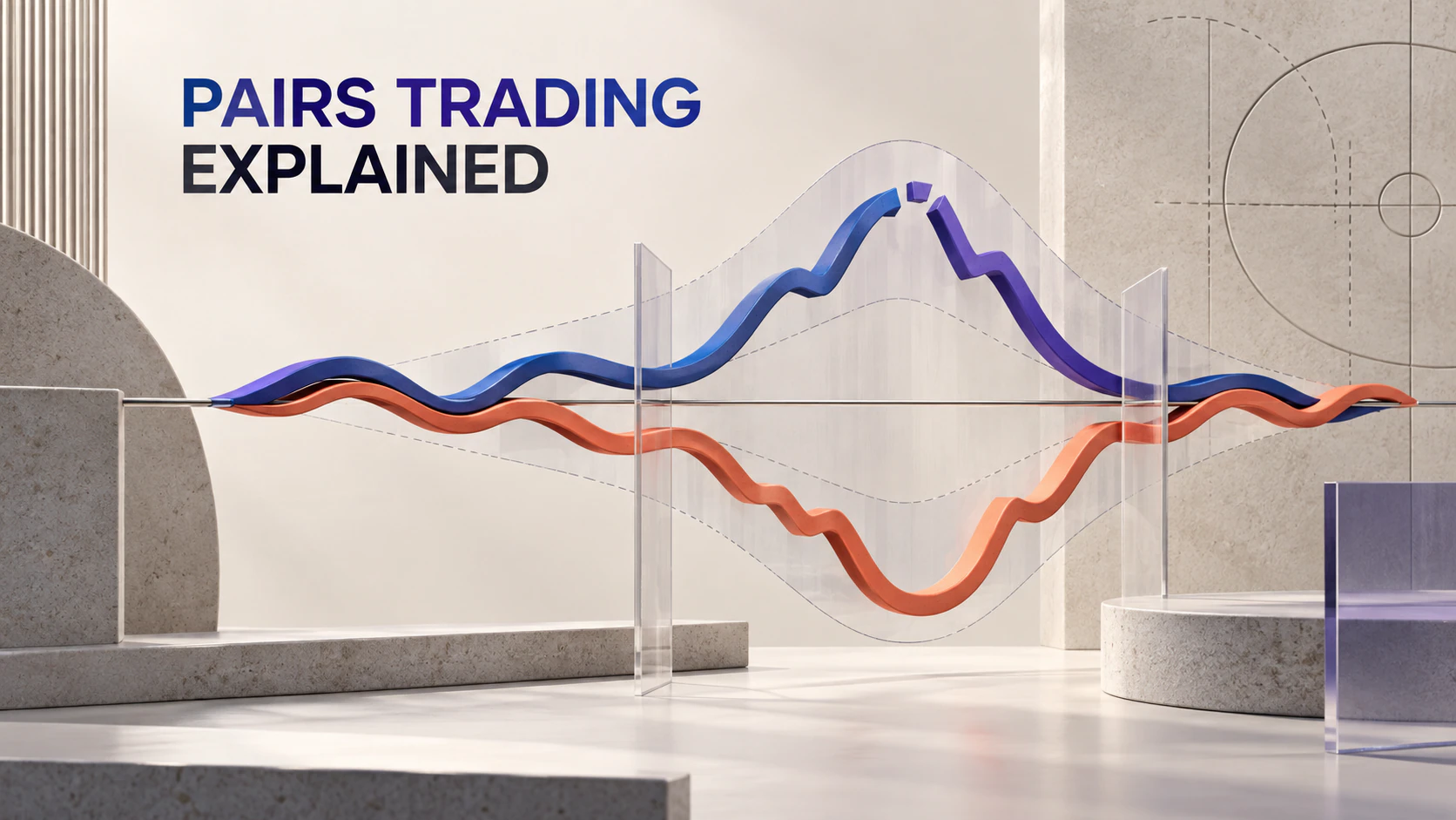
Pairs trading is a relative-value strategy that focuses on the relationship between two assets rather than predicting the overall direction of the market. The strategy seeks two securities whose prices have historically maintained a stable connection. When that relationship deviates significantly from its normal range, a trader buys the relatively undervalued asset and shorts the relatively overvalued one, anticipating that the gap will eventually narrow.
For example, two companies operating in the same industry may respond to similar economic conditions, input costs and demand patterns. If one stock rises sharply while the other lags without an obvious fundamental reason, a pairs trader may short the stronger stock and buy the weaker one. The position may become profitable if their relative valuations converge.
The central challenge is determining whether the observed relationship is genuinely stable. Similar-looking price charts alone are not sufficient.
Correlation and Cointegration
Correlation measures whether two assets have tended to move in the same or opposite direction during a particular period. It is useful for identifying potential pairs, but a high correlation does not prove that the distance between their prices will return to a long-term equilibrium.
Cointegration addresses a different question. Two price series may individually trend over time while a particular linear combination of them remains relatively stable. If the resulting residual or spread displays mean-reverting behavior, it may provide a stronger statistical foundation for a trading strategy.
Two assets can therefore be highly correlated without being cointegrated. A strategy based only on correlation may mistake temporary synchronization for a durable relationship.
Spread, Hedge Ratio and Z-Score
A pairs strategy normally begins by estimating a hedge ratio. If the prices of assets A and B are represented by PA and PB, and the hedge ratio is β, the spread can be expressed as:
Spread = PA − β × PB
The hedge ratio determines the relative size of the two positions. It does not have to be one-to-one. Traders may estimate it through linear regression, rolling regression or a dynamic model, and may further adjust the positions according to capital, volatility or risk exposure.
The spread is often standardized with a z-score:
Z-score = (Current spread − Historical mean) ÷ Historical standard deviation
A strongly positive z-score may trigger a short-spread position: short asset A and buy the appropriate quantity of asset B. A strongly negative reading may produce the opposite trade. The position is usually closed when the spread approaches its estimated mean.
Entry and exit thresholds should not be selected simply because they generated the best historical result. Repeatedly optimizing thresholds, lookback periods and holding rules can create an overfitted strategy that performs poorly on new data.
Common Pairs Trading Models
The distance method is one of the simplest approaches. Prices are normalized, and assets with similar historical paths are selected as potential pairs. This method is intuitive and easy to implement, but it provides limited evidence that the relationship represents a persistent equilibrium.
Cointegration models test whether a stable linear combination exists between non-stationary price series. The Engle–Granger approach is commonly applied to a pair of variables, while the Johansen method can examine systems involving multiple assets. Statistical significance, however, does not automatically imply economic logic or future stability.
Time-series models can describe how the spread evolves. Autoregressive models may estimate the speed of mean reversion, while the spread’s half-life approximates how long a deviation could take to decay. A slowly reverting spread may tie up capital for too long, while a very fast one may offer too little profit after execution costs.
A Kalman filter can estimate a hedge ratio that changes over time. This flexibility may help when the relationship between two assets evolves, but it also introduces additional parameters and model risk. A model that reacts too aggressively to short-term noise can produce unstable signals and excessive turnover.
Machine learning may assist with pair selection, market-regime classification or spread forecasting. It does not remove the strategy’s core risks. Data leakage, weak out-of-sample performance and limited interpretability can make a complex model appear more reliable than it really is.
Building a Pairs Trading Process
The process usually begins with an economically coherent universe, such as companies in the same industry, bonds with similar characteristics, related commodities or structurally comparable funds. Liquidity, correlation, cointegration and spread stability can then be used to narrow the list of candidates.
The strategy requires explicit entry, exit, stop-loss and maximum holding-period rules. A realistic backtest must include commissions, bid–ask spreads, slippage, financing expenses, stock-borrowing costs and possible delays between the two executions. Signals must also be calculated only from information that would have been available at the time.
Evaluation should extend beyond total return. Maximum drawdown, win rate, payoff ratio, turnover, average holding period, tail losses and performance across different market regimes all provide important context. Rolling analysis and genuinely independent out-of-sample testing are particularly valuable for assessing whether a relationship remains dependable.
The Principal Risks
Relationship breakdown is the defining risk. Changes in company fundamentals, mergers, regulation, index membership or industry structure can move the assets into a new equilibrium. Waiting for the old relationship to return may then deepen the loss rather than resolve it.
Model risk is also significant. Results can change materially when the sample period, hedge ratio or trading thresholds are adjusted. An apparently strong relationship may be an accidental product of data mining.
Execution risk can erode a theoretical advantage. If both legs cannot be filled simultaneously, the portfolio becomes temporarily exposed to market direction. Declining liquidity, widening spreads or the recall of borrowed shares can further damage performance.
Pairs trading is not automatically market-neutral. Two positions with equal monetary values may still have different betas, volatilities, sector sensitivities and liquidity profiles. During market stress, correlations can change abruptly, and multiple pairs that once appeared diversified may lose money at the same time.
The appeal of pairs trading lies in shifting attention from outright market forecasts to relative relationships. However, mean reversion is a hypothesis that must be continually tested, not a guaranteed outcome. A robust implementation must evaluate whether the relationship is still valid and manage uncertainty through position limits, structural stop rules, realistic cost assumptions and diversification across genuinely independent opportunities.